17. Creating knowledge graphs from unstructured text

17.1. Main Objectives
If you ever had to do a literature search for a project, you probably can appreciate the great effort behind traversing
the ever-expanding volumes of texts and trying to organise the extracted information.
In the past two decades, noticeable progress has been made, harnessing the power of machine-learning (ML) and
artificial intelligence (AI) based approaches to extract knowledge from large corpora of scientific literature.
Modern ML algorithms aim to identify, extract, and store important information from unstructured text.
Among the most popular structured representations, knowledge graphs, in the form of RDF linked data graphs are rapidly
becoming a dominant form. This is chiefly due to it being a favourite form of active metadata and FAIR data.
In simplified terms, the overall pipeline for information extraction can be broken down in the following key steps:
Collecting the text data and assembling the data corpus
Performing entity disambiguation using a technique such as co-reference resolution
Performing entity recognition and named entity linking (NER step)
Performing relationship detection and extraction
Creating and storing the data in a knowledge graph (an RDF linked data graph in our example).
17.2. Graphical Overview
This recipe will cover the highlighted topics

Fig. 17.1 Overview of natural language processing to knowledge graph creation workflow
Recipe dependency:
Skill dependency:
Programming knowledge
Python
Technical dependency
Python environment
Semantic Web technologies
Actions.Objectives.Tasks |
Input |
Output |
|---|---|---|
17.3. Tools
The table below lists the software that is used to execute the examples in this recipe.
Software |
Description |
|---|---|
The biopython project is an open-source collection of non-commercial Python tools for computational biology and bioinformatics, created by an international association of developers |
|
Spacy is a beginner level industry strength natural language processing library |
|
A multi-lingual approach to AllenNLP CoReference Resolution along with a wrapper for spaCy |
|
REBEL is a seq2seq model that simplifies Relation Extraction |
|
RDFLib is a Python library for working with RDF, a framework for representing information |
|
NetworkX is a Python package for the creation, manipulation, and study of the structure, dynamics, and functions of complex networks. |
|
Matplotlib is a comprehensive library for creating static, animated, and interactive visualizations in Python. |
17.4. Generation of textual corpora
First, one collects the text to extract the data from. Text may come from the internal documents, articles, online content (web scraping), patents, or even be a result of picture descriptions produced by image-to-text algorithms.
In our example, we created a dataset of articles’ abstracts (corpora) on the topic “cardiac amyloidosis”. In the biological domain, articles can be collected from the PubMed database using biopython. For the sake of simplicity, we retained only the first 5 articles that come up in the search.
#importing libraries
from Bio import Entrez

def search(query, max_papers=5):
    """
    Get IDs of papers on the given topic from the pubmed database.
    """
    handle = Entrez.esearch(
        db='pubmed',
        sort='relevance',
        retmax=max_papers,
        retmode='xml',
        term=query
    )
    results = Entrez.read(handle)
    return results

def fetch_details(id_list):
    """
    Get details on each paper (including the abstract).
    """
    ids = ','.join(id_list)
    handle = Entrez.efetch(
        db='pubmed',
        retmode='xml',
        id=ids
    )
    results = Entrez.read(handle)
    return results

results = search('cardiac amyloidosis')
id_list = results['IdList']
papers = fetch_details(id_list)
17.5. Entity disambiguation using co-reference resolution
The text corpus prepared in the previous step is now processed to replace all ambiguous words found in a sentence so
that the text does not need any extra context to be understood.
Although a number of approaches to perform this task exists, one of the most recently developed is a method known as
crosslingual coreference from the
spaCy python library 1.
spaCy is a python library providing a comprehensive yet accessible way to
create pipelines for natural language processing.
In a nutshell, applying this procedure will, for example, replace personal pronouns with a referred person’s name.
import spacy
import crosslingual_coreference

DEVICE = -1 # Number of the GPU, -1 if want to use CPU

# Add coreference resolution model
coref = spacy.load(
    'en_core_web_sm',
    disable=['ner', 'tagger', 'parser', 'attribute_ruler', 'lemmatizer']
)
coref.add_pipe(
    "xx_coref",
    config={"chunk_size": 2500, "chunk_overlap": 2, "device": DEVICE}
)
17.6. Entity recognition and named entity linking
The next step is known as Named Entity Recognition (NER). Here, we want to detect and extract all domain relevant entities from the sentences. Depending on the use case, one may have to specifically train a model to recognise entities of a specific type. For example, in this tutorial, one can find a way to train a model to recognise some entities from a biomedical domain. However, the spaCy library also provides a number of pre-trained models and, we will be using those in our example.
Following the entity recognition, one needs to standardise the entities and map them to an existing controlled terminology/ontology.
The process is known as Entity Linking (EL).
With this step, entities recognized from the text are mapped to one or more corresponding unique resolvable identifiers
from a target knowledge base, for example, Wikipedia or semantic resource (e.g. an ontology such as
disease ontology) 3.
One may also use resolvable identifiers minted by databases and relevant to the specific topic of the texts.
In this example, we will map our entities to the NCI Thesaurus and for simplicity, we will by default choose the first match as a mapping.
Warning
Note, that in principle that is not always the best choice and one may wish to use different similarity metrics to identify the best matching term in the ontology.
Note
A mapping to Wikipedia terms is demonstrated in this tutorial,
17.7. Relationship Extraction
Following the step of entity linking, we now need to extract the relationships between the identified entities. This is necessary to be able to generate canonical RDF triples, also known as RDF subject predicate object statements, and build a knowledge graph, To perform the relation identification, we will use the python Rebel project, which is also available as a spaCy component, and allows extracting both entities and relations in one step 2. We will now use it in our pipeline.
To implement our approach of linking the entities to NCIT, we can rewrite the set_annotations function from the Rebel
code as specified here
and alter the call_wiki_api function into call_ncit function.
import pandas as pd
import requests

def call_ncit_api(item):
  """
  Get the first mapping term from the NCIT
  """
  try:
    url = f"https://www.ebi.ac.uk/ols/api/search?q={item}&ontology=ncit"
    data = pd.DataFrame(requests.get(url).json().get('response').get('docs'))
    # Return the first id (A simplistic non-perfect way for mapping)
    return data["label"][0]
  except:
    return 'id-less'
After redefining the Rebel spaCy component, we include it into our pipeline:
rel_ext = spacy.load(
    'en_core_web_sm',
    disable=['ner', 'lemmatizer', 'attribute_rules', 'tagger']
)
rel_ext.add_pipe(
    "rebel",
    config={
        'device':DEVICE, # Number of the GPU, -1 if want to use CPU
        'model_name':'Babelscape/rebel-large' # Model used
    }
)
Now, we can test the pipeline on two simple sentences:
input_text = "High fever is very dangerous. It can be treated with paracetamol."

#coreference model
coref_text = coref(input_text)._.resolved_text
print(coref_text)
#output: 'High fever is very dangerous. High fever can be treated with paracetamol.'

#entity and relations extraction
doc = rel_ext(coref_text)

for value, rel_dict in doc._.rel.items():
    print(f"{value}: {rel_dict}")

#output:
#0440ea848947d2677bc11443f99f20f67ce0a1bc: {'relation': 'subclass of', 'head_span': {'text': 'High fever', 'id': 'High Grade Fever'}, 'tail_span': {'text': 'dangerous', 'id': 'DRRI-2 - A: Dangerous Military Duties'}}
#8aa25d264897bd007d389890b2239c2b9c07fa0b: {'relation': 'drug used for treatment', 'head_span': {'text': 'High fever', 'id': 'High Grade Fever'}, 'tail_span': {'text': 'paracetamol', 'id': 'Acetaminophen Measurement'}}
#d91bef9bfc94439523675b5d6a62e1f4635c0cdd: {'relation': 'medical condition treated', 'head_span': {'text': 'paracetamol', 'id': 'Acetaminophen Measurement'}, 'tail_span': {'text': 'High fever', 'id': 'High Grade Fever'}}
Following the disambiguation step (using co-reference), the “it” pronoun in the second sentence is replaced by the
unambiguous “High fever” entity.
After that step, the Rebel model extracted the subject, relation, object triples and mapped them to the NCIT model.
Warning
Note that the automatic mapping is far from perfect. For example, the entity ‘dangerous’ was mapped to the ‘DRRI-2 - A: Dangerous Military Duties’ in NCIT. This is a consequence of our unrefined mapping procedure in which, for simplicity, the default selection of the first result for the term in the NCIT database was done. To improve over this simplistic approach, one would need to develop a more advanced mapping heuristic, but this is out of the scope of this recipe. Having said that, a key learning point is that a ‘man in the loop’ approach is probably still needed to review the mapping resulting from such automated approaches.
17.8. Storing the results
The final subject, predicate, object triples can either be stored as a labeled property graph or as an RDF graph.
Here, we will outline an approach to store the results as an RDF graph by using the python rdflib library.
rdflib allows the creation of entities with known URIs with the URIRef command.
Also, one can create a custom namespace with new entities and relations.
Note
For our audience interested in labeled property graphs, the guidelines to store the results as a neo4j labeled property graph are available from this tutorial.
from rdflib import Graph
from rdflib import URIRef, BNode, Literal, Namespace
import json

def Capitalise_underscore(relation):
  """
  Write the relations in Capitalized_And_Underscored_form
  """
  return relation.capitalize().replace(' ','_')

def ncit_iri(item):
  """
  Get an iri of the first matching term from NCIT
  """
  try:
    url = f"https://www.ebi.ac.uk/ols/api/search?q={item}&ontology=ncit"
    data = pd.DataFrame(requests.get(url).json().get('response').get('docs'))
    # Return the first id
    return data["iri"][0]
  except:
    return 'id-less'

#create the graph
g=Graph()
EX = Namespace('http://example.org./')

#dataframe storing the trios for visual clarity
relations = pd.DataFrame()

for i, paper in enumerate(papers['PubmedArticle']):
    print("{}) {}".format(i+1, paper['MedlineCitation']['Article']['ArticleTitle']))
    #get abstract
    abstract_text_json = json.dumps(papers['PubmedArticle'][i]['MedlineCitation']['Article']['Abstract']['AbstractText'])
    abstract_text = ' '.join(json.loads(abstract_text_json))

    #take through coreference model
    coref_text = coref(abstract_text)._.resolved_text

    #entity extraction and linking
    doc = rel_ext(coref_text)

    #adding trios to the graph
    for value, rel_dict in doc._.rel.items():
      subject_iri = ncit_iri(rel_dict['head_span']['text'])
      object_iri = ncit_iri(rel_dict['head_span']['text'])
      if subject_iri != 'id-less':
        subj = URIRef(subject_iri)
      else:
        subj = EX[rel_dict['head_span']['text']]
      if object_iri != 'id-less':
        obj = URIRef(object_iri)
      else:
        subj = EX[rel_dict['head_span']['text']]
      pred = EX[Capitalise_underscore(rel_dict['relation'])]
      g.add((subj, pred, obj))

    df = pd.DataFrame.from_dict(doc._.rel).transpose()
    df['subject_text'] = df.head_span.apply(lambda x: x['text'])
    df['subject_id'] = df.head_span.apply(lambda x: x['id'])
    df['object_text'] = df.tail_span.apply(lambda x: x['text'])
    df['object_id'] = df.tail_span.apply(lambda x: x['id'])

    df.drop(["head_span", "tail_span"], axis = 1, inplace=True)

    relations = pd.concat([relations, df])
Finally, we can export the resulting graph in turtle (.ttl) format … library.
g.serialize(format = 'ttl')
…and visualise it using the well known networkx python library and matplotlib library.
from matplotlib import colors as mcolors
from matplotlib.lines import Line2D

def make_proxy(clr, mappable, **kwargs):
    return Line2D([0, 1], [0, 1], color=clr, **kwargs)

#for id-less set the identified entity as the id
relations.replace(['id-less'], [None], inplace=True)
relations['subject_id'] = relations['subject_id'].fillna(relations['subject_text'])
relations['object_id'] = relations['object_id'].fillna(relations['object_text'])

#bring all entities to upper case
relations = relations.applymap(lambda s:s.upper())
relations['relation'] = relations['relation'].apply(lambda s:s.lower())
relations['relation']=pd.Categorical(relations['relation'])


#select colors for edges
clrs = ['b', 'g', 'r', 'c', 'm', 'y', 'k', 'aqua', 'brown', 'darkgray',
        'orange', 'burlywood', 'cadetblue', 'chartreuse',
        'chocolate', 'coral','cornflowerblue','cornsilk','crimson']
#map relations to colors
color_map = dict(zip(relations['relation'].unique(), clrs))
#create the list of edge colors
relations['edge_colors'] = relations["relation"].apply(lambda x: color_map[x])
graph = ntx.from_pandas_edgelist(relations, "subject_id", "object_id", edge_attr="edge_colors", create_using=ntx.MultiDiGraph())

## PLOT
plt.figure(figsize=(20, 20))
posn = ntx.shell_layout(graph)

colors = ntx.get_edge_attributes(graph,'edge_colors').values()

##add graph elements
h1 = ntx.draw_networkx_nodes(graph, pos=posn, node_color = 'lightgray', node_size = 300)
h2 = ntx.draw_networkx_edges(graph, pos=posn, width=1, edge_color=colors)
h3 = ntx.draw_networkx_labels(graph, pos=posn, font_size=10)

# generate proxies
proxies = [make_proxy(clr, h2, lw=5) for clr in color_map.values()]
#create legend labels
labels = color_map.keys()
plt.legend(proxies, labels)
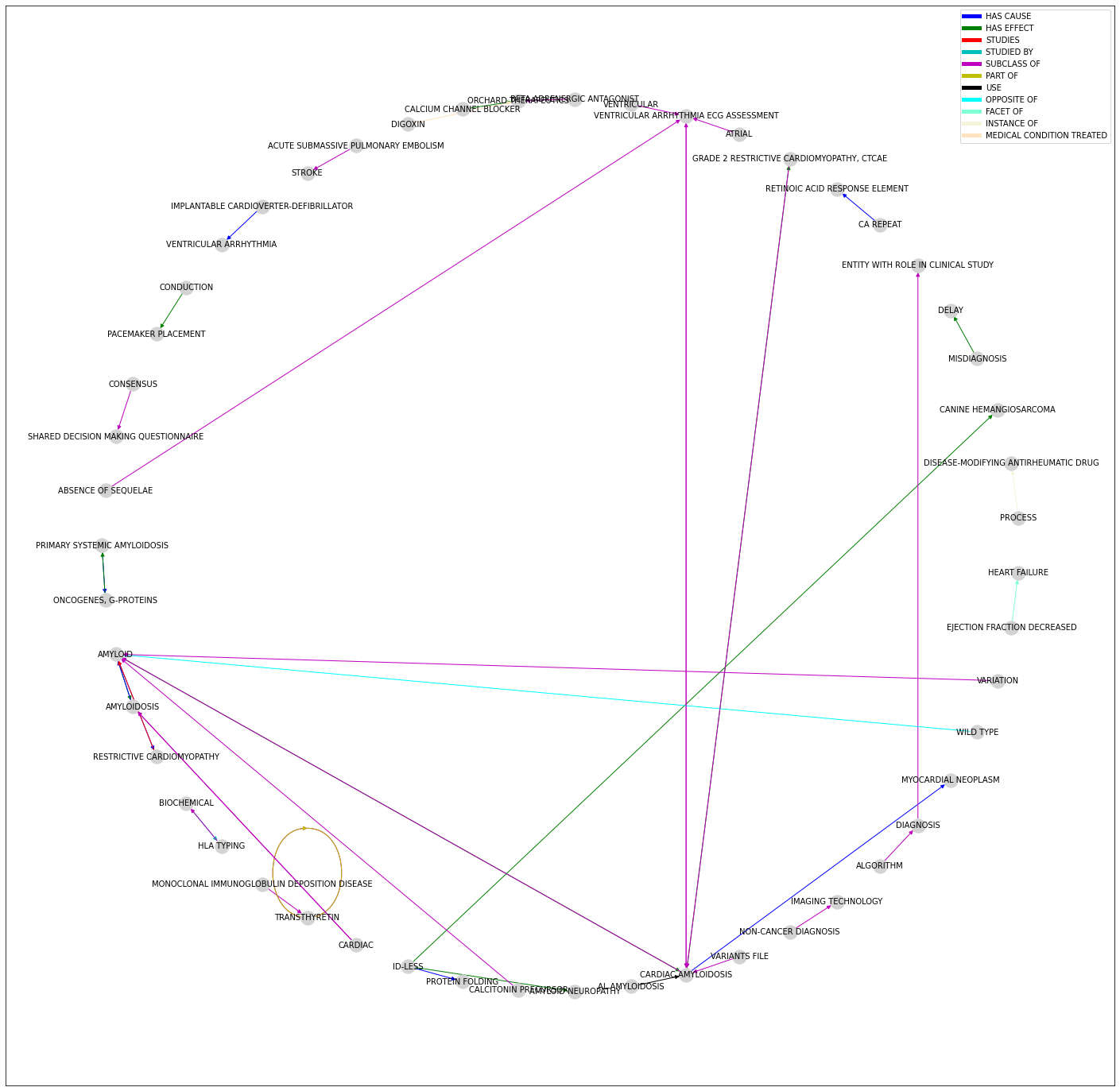
Fig. 17.2 Viewing the knowledge graph with networks and matplotlib
17.9. Conclusion
Modern AI/ML algorithms allow processing large corpus of unstructured text and extract information to structure it. For instance, information can be organised in a form of knowledge graphs, e.g. RDF linked open data (LOD) graphs. The present document provides a typical text processing pipeline to achieve this task, even if in a simplified form. In more realistic cases, large text corpora will require more advanced techniques to be deployed, from model training to the development of specific algorithms, and the inclusion of expert curators to assist in the creation of the final knowledge graphs. Still, we hope this will provide our readership with a basic understanding of the techniques available to move from unstructured text to generating knowledge graphs.
Warning
So we have now an RDF graph but does it mean it is properly FAIR? Well, not quite. First, the graph is not findable as it it. Furthermore, it lacks a link to a licence, let alone a machine readable license. Provenance metadata is also missing and turning the graph into a named graph with a stable resolvable identifier constitute the additional steps required to turn this graph into a FAIR digital object of a reasonable maturity state.
17.9.1. What to read next?
FAIRsharing records appearing in this recipe:
17.10. References
references
- 1
Crosslingual coreference. URL: https://spacy.io/universe/project/crosslingualcoreference.
Pere-Lluís Huguet Cabot and Roberto Navigli. REBEL: relation extraction by end-to-end language generation. In Findings of the Association for Computational Linguistics: EMNLP 2021, 2370–2381. Punta Cana, Dominican Republic, November 2021. Association for Computational Linguistics. URL: https://aclanthology.org/2021.findings-emnlp.204.
- 3
L. M. Schriml, J. B. Munro, M. Schor, D. Olley, C. McCracken, V. Felix, J. A. Baron, R. Jackson, S. M. Bello, C. Bearer, R. Lichenstein, K. Bisordi, N. C. Dialo, M. Giglio, and C. Greene. The Human Disease Ontology 2022 update. Nucleic Acids Res, 50(D1):D1255–D1261, Jan 2022.
17.11. Authors
Authors
Name |
ORCID |
Affiliation |
Type |
ELIXIR Node |
Contribution |
|---|---|---|---|---|---|
Bayer AG |
Writing - Original Draft |
||||
University of Oxford |
|
Review, Writing, Conceptualization |